4. Use Autoencoder to implement anomaly detection.

Use Autoencoder to implement anomaly detection. Build the model by using: 

a. Import required libraries 
b. Upload / access the dataset 
c. Encoder converts it into latent representation 
d. Decoder networks convert it back to the original input 
e. Compile the models with Optimizer, Loss, and Evaluation Metrics

Download Writeup here

Let's build the simplest possible autoencoder

We'll start simple, with a single fully-connected neural layer as encoder and as decoder:

import keras
from keras import layers
# This is the size of our encoded representations
encoding_dim = 32  # 32 floats -> compression of factor 24.5, assuming the input is 784 floats
# This is our input image
input_img = keras.Input(shape=(784,))
# "encoded" is the encoded representation of the input
encoded = layers.Dense(encoding_dim, activation='relu')(input_img)
# "decoded" is the lossy reconstruction of the input
decoded = layers.Dense(784, activation='sigmoid')(encoded)
# This model maps an input to its reconstruction
autoencoder = keras.Model(input_img, decoded)

Let's also create a separate encoder model:

# This model maps an input to its encoded representation
encoder = keras.Model(input_img, encoded)

As well as the decoder model:

# This is our encoded (32-dimensional) input
encoded_input = keras.Input(shape=(encoding_dim,))
# Retrieve the last layer of the autoencoder model
decoder_layer = autoencoder.layers[-1]
# Create the decoder model
decoder = keras.Model(encoded_input, decoder_layer(encoded_input))

Now let's train our autoencoder to reconstruct MNIST digits.
First, we'll configure our model to use a per-pixel binary crossentropy loss, and the Adam optimizer:

autoencoder.compile(optimizer='adam', loss='binary_crossentropy')

Let's prepare our input data. We're using MNIST digits, and we're discarding the labels (since we're only interested in encoding/decoding the input images).

from keras.datasets import mnist
import numpy as np
(x_train, _), (x_test, _) = mnist.load_data()

We will normalize all values between 0 and 1 and we will flatten the 28x28 images into vectors of size 784.

x_train = x_train.astype('float32') / 255.
x_test = x_test.astype('float32') / 255.
x_train = x_train.reshape((len(x_train), np.prod(x_train.shape[1:])))
x_test = x_test.reshape((len(x_test), np.prod(x_test.shape[1:])))
print(x_train.shape)
print(x_test.shape)

Now let's train our autoencoder for 50 epochs:

autoencoder.fit(x_train, x_train,
                epochs=50,
                batch_size=256,
                shuffle=True,
                validation_data=(x_test, x_test))

After 50 epochs, the autoencoder seems to reach a stable train/validation loss value of about 0.09. We can try to visualize the reconstructed inputs and the encoded representations. We will use Matplotlib.

# Encode and decode some digits
# Note that we take them from the *test* set
encoded_imgs = encoder.predict(x_test)
decoded_imgs = decoder.predict(encoded_imgs)

# Use Matplotlib

import matplotlib.pyplot as plt
n = 10  # How many digits we will display
plt.figure(figsize=(20, 4))
for i in range(n):
    # Display original
    ax = plt.subplot(2, n, i + 1)
    plt.imshow(x_test[i].reshape(28, 28))
    plt.gray()
    ax.get_xaxis().set_visible(False)
    ax.get_yaxis().set_visible(False)
    # Display reconstruction
    ax = plt.subplot(2, n, i + 1 + n)
    plt.imshow(decoded_imgs[i].reshape(28, 28))
    plt.gray()
    ax.get_xaxis().set_visible(False)
    ax.get_yaxis().set_visible(False)
plt.show()

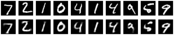
Here's what we get. The top row is the original digits, and the bottom row is the reconstructed digits. We are losing quite a bit of detail with this basic approach.