| |
| # # Title of Assignment-2: |
| # Implementing Feedforward neural networks with Keras and TensorFlow |
| # a. Import the necessary packages |
| # b. Load the training and testing data (MNIST) |
| # c. Define the network architecture using Keras |
| # d. Train the model using SGD |
| # e. Evaluate the network |
| # f. Plot the training loss and accuracy |
| # |
|
|
| # # Importing libraries |
|
|
| # In[1]: |
|
|
|
|
| #importing necessary libraries |
| import tensorflow as tf |
| from tensorflow import keras |
|
|
|
|
| # In[2]: |
|
|
|
|
| import pandas as pd |
| import numpy as np |
| import matplotlib.pyplot as plt |
| import random |
| get_ipython().run_line_magic('matplotlib', 'inline') |
|
|
|
|
| # # Loading and preparing the data |
|
|
| # MNIST stands for “Modified National Institute of Standards and Technology”. |
| # It is a dataset of 70,000 handwritten images. Each image is of 28x28 pixels |
| # i.e. about 784 features. Each feature represents only one pixel’s intensity i.e. from 0(white) to 255(black). |
| # This database is further divided into 60,000 training and 10,000 testing images. |
|
|
| # In[3]: |
|
|
|
|
| #import dataset and split into train and test data |
| mnist = tf.keras.datasets.mnist |
| (x_train, y_train), (x_test, y_test) = mnist.load_data() |
|
|
|
|
| # In[4]: |
|
|
|
|
| #to see length of training dataset |
| len(x_train) |
|
|
|
|
| # In[5]: |
|
|
|
|
| ##to see length of testing dataset |
| len(x_test) |
|
|
|
|
| # In[6]: |
|
|
|
|
| #shape of training dataset 60,000 images having 28*28 size |
| x_train.shape |
|
|
|
|
| # In[7]: |
|
|
|
|
| #shape of testing dataset 10,000 images having 28*28 size |
| x_test.shape |
|
|
|
|
| # In[12]: |
|
|
|
|
|
|
| x_train[0] |
|
|
|
|
| # In[8]: |
|
|
|
|
| #to see how first image look |
| plt.matshow(x_train[0]) |
|
|
|
|
| # In[9]: |
|
|
|
|
| #normalize the images by scaling pixel intensities to the range 0,1 |
|
|
| x_train = x_train / 255 |
| x_test = x_test / 255 |
|
|
|
|
| # In[10]: |
|
|
|
|
| x_train[0] |
|
|
|
|
| # In[ ]: |
|
|
|
|
| #Define the network architecture using Keras |
|
|
|
|
| # # Creating the model |
| # |
|
|
| # The ReLU function is one of the most popular activation functions. |
| # It stands for “rectified linear unit”. Mathematically this function is defined as: |
| # y = max(0,x)The ReLU function returns “0” if the input is negative and is linear if |
| # the input is positive. |
| # |
| # The softmax function is another activation function. |
| # It changes input values into values that reach from 0 to 1. |
|
|
| # In[11]: |
|
|
|
|
| model = keras.Sequential([ |
| keras.layers.Flatten(input_shape=(28, 28)), |
| keras.layers.Dense(128, activation='relu'), |
| keras.layers.Dense(10, activation='softmax') |
| ]) |
|
|
|
|
| # In[12]: |
|
|
|
|
| model.summary() |
|
|
|
|
| # # Compile the model |
|
|
| # In[13]: |
|
|
|
|
| model.compile(optimizer='sgd', |
| loss='sparse_categorical_crossentropy', |
| metrics=['accuracy']) |
|
|
|
|
| # # Train the model |
|
|
| # In[14]: |
|
|
|
|
| history=model.fit(x_train, y_train,validation_data=(x_test,y_test),epochs=10) |
|
|
|
|
| # # Evaluate the model |
|
|
| # In[15]: |
|
|
|
|
| test_loss,test_acc=model.evaluate(x_test,y_test) |
| print("Loss=%.3f" %test_loss) |
| print("Accuracy=%.3f" %test_acc) |
|
|
|
|
| # # Making Prediction on New Data |
|
|
| # In[18]: |
|
|
|
|
| n=random.randint(0,9999) |
| plt.imshow(x_test[n]) |
| plt.show() |
|
|
|
|
| # |
|
|
| # In[19]: |
|
|
|
|
| #we use predict() on new data |
| predicted_value=model.predict(x_test) |
| print("Handwritten number in the image is= %d" %np.argmax(predicted_value[n])) |
|
|
|
|
| # # Plot graph for Accuracy and Loss |
|
|
| # In[20]: |
|
|
|
|
| get_ipython().run_line_magic('pinfo2', 'history.history') |
|
|
|
|
| # In[21]: |
|
|
|
|
| history.history.keys() |
|
|
|
|
| # In[22]: |
|
|
|
|
| plt.plot(history.history['accuracy']) |
| plt.plot(history.history['val_accuracy']) |
| plt.title('model accuracy') |
| plt.ylabel('accuracy') |
| plt.xlabel('epoch') |
| plt.legend(['Train', 'Validation'], loc='upper left') |
| plt.show() |
|
|
|
|
| # graph representing the model’s accuracy |
|
|
| # In[23]: |
|
|
|
|
| plt.plot(history.history['loss']) |
| plt.plot(history.history['val_loss']) |
| plt.title('model loss') |
| plt.ylabel('loss') |
| plt.xlabel('epoch') |
| plt.legend(['Train', 'Validation'], loc='upper left') |
| plt.show() |
|
|
|
|
| # graph represents the model’s loss |
|
|
| # In[24]: |
|
|
|
|
| plt.plot(history.history['accuracy']) |
| plt.plot(history.history['val_accuracy']) |
| plt.plot(history.history['loss']) |
| plt.plot(history.history['val_loss']) |
| plt.title('Training Loss and accuracy') |
| plt.ylabel('accuracy/Loss') |
| plt.xlabel('epoch') |
| plt.legend(['accuracy', 'val_accuracy','loss','val_loss']) |
| plt.show() |
|
|
|
|
| # Conclusion: With above code We can see, that throughout the epochs, our model accuracy |
| # increases and our model loss decreases,that is good since our model gains confidence |
| # with its predictions. |
| # |
| # 1. The two losses (loss and val_loss) are decreasing and the accuracy |
| # (accuracy and val_accuracy)are increasing. |
| # So this indicates the model is trained in a good way. |
| # |
| # 2. The val_accuracy is the measure of how good the predictions of your model are. |
| # So In this case, it looks like the model is well trained after 10 epochs |
|
|
| # In[50]: |
|
|
|
|
| #pwd |
|
|
|
|
| # # Save the model |
|
|
| # In[25]: |
|
|
|
|
| keras_model_path='C:\\Users\\admin' |
| model.save(keras_model_path) |
|
|
|
|
| # In[26]: |
|
|
|
|
| #use the save model |
| restored_keras_model = tf.keras.models.load_model(keras_model_path) |
|
|
|
|
| # In[ ]: |
Comments
Post a Comment